Deep Dive into Diffusion Models

This blog is my learning notes on the Diffusion Models, which is the state-of-art generative models. This blog will cover that is the diffusion models, how to use diffusion models to generate image, text-to-image, video. It also cover lagnuage diffusion model.

What is the Diffusion Models?

Diffusion Model is know

Diffusion Models in nutshell

Let’s first create a very simple diffusion model based on MNIST data. (Full code is available here)

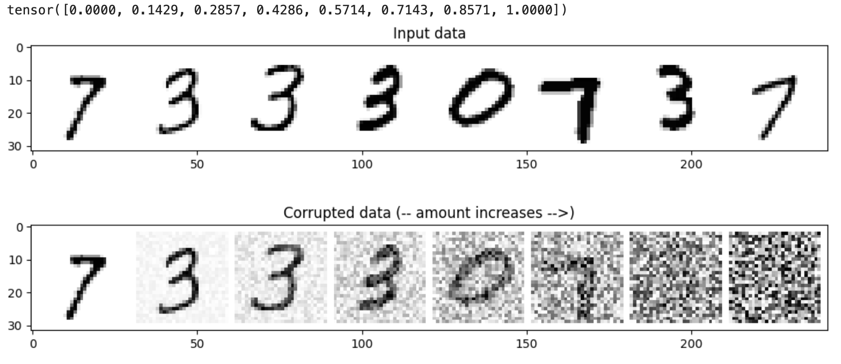
The central idea is to take each training image and to corrupt it using a multi-step noise process to transform it into a sample from Gaussian distribution. A deep neural network is then trained to invert this process, and once trained the network can then generate new images starting with samples from Gaussian as input

Deep LearningFoundations and Concepts

The corrupt process is defined as:

def corrupt(x, amount):
    """
    corrupt the input `x` by mixing it with noise
    x: (B, 1, 28, 28)
    amount: (B) different amount of noise for different samples
    """
    noise = torch.rand_like(x)
    amount = amount.view(-1, 1, 1, 1)
    return x * (1 - amount) + noise * amount

We take a batch of image in, and corrupt the image the according to different level of noise.

Figure 1: Corrupt images with differnt level of noise.

After we get images and corresponding corrupted images, we need to create a neural network to invert this process, which mean we need the neural network take the noise image in, get the de-noised(real) image out. And we want those two as close as possible. So, the loss function \(\mathcal{L}\) is:

\[ \mathcal{L}(\theta) = \sum_{i = 1}^{N}\| f_\theta(\hat{\mathrm{x}}_i) - \mathrm{x}_i \|^2 \tag{1}\]

which is the Mean Square Loss.

So, there are different types of neural network, which one should we choose? Since we need the output has same shape as the input, the U-Net(Ronneberger, Fischer, and Brox 2015) is perfect choice.

U-Net

Now, we got everything we need to trained a neural network, data, model, loss function, let’s start training!!

batch_size = 128
train_dataloader = DataLoader(dataset, batch_size=batch_size, shuffle=True)
epochs = 10

net = UNet()  # This UNet is trained to predict the original image from the corrupted image
criterion = nn.MSELoss()
optimizer = torch.optim.Adam(net.parameters(), lr=1e-3)

for epoch in range(epochs):
    for x, _ in tqdm(train_dataloader):
        noise_amount = torch.rand(x.shape[0]) # Random Generate some noise level[0, 1] add to image x
        noisy_x = corrupt(x, noise_amount) # Corrput the image

        pred = net(noisy_x) # NN predict what the de-noised image x
        loss = criterion(pred, x) # Compare 

        # Optimize
        optimizer.zero_grad()
        loss.backward()
        optimizer.step()

After we trained the model for 10 epochs, we can see that it predict not-bad output.

Figure 2: Result of one pass U-Net model

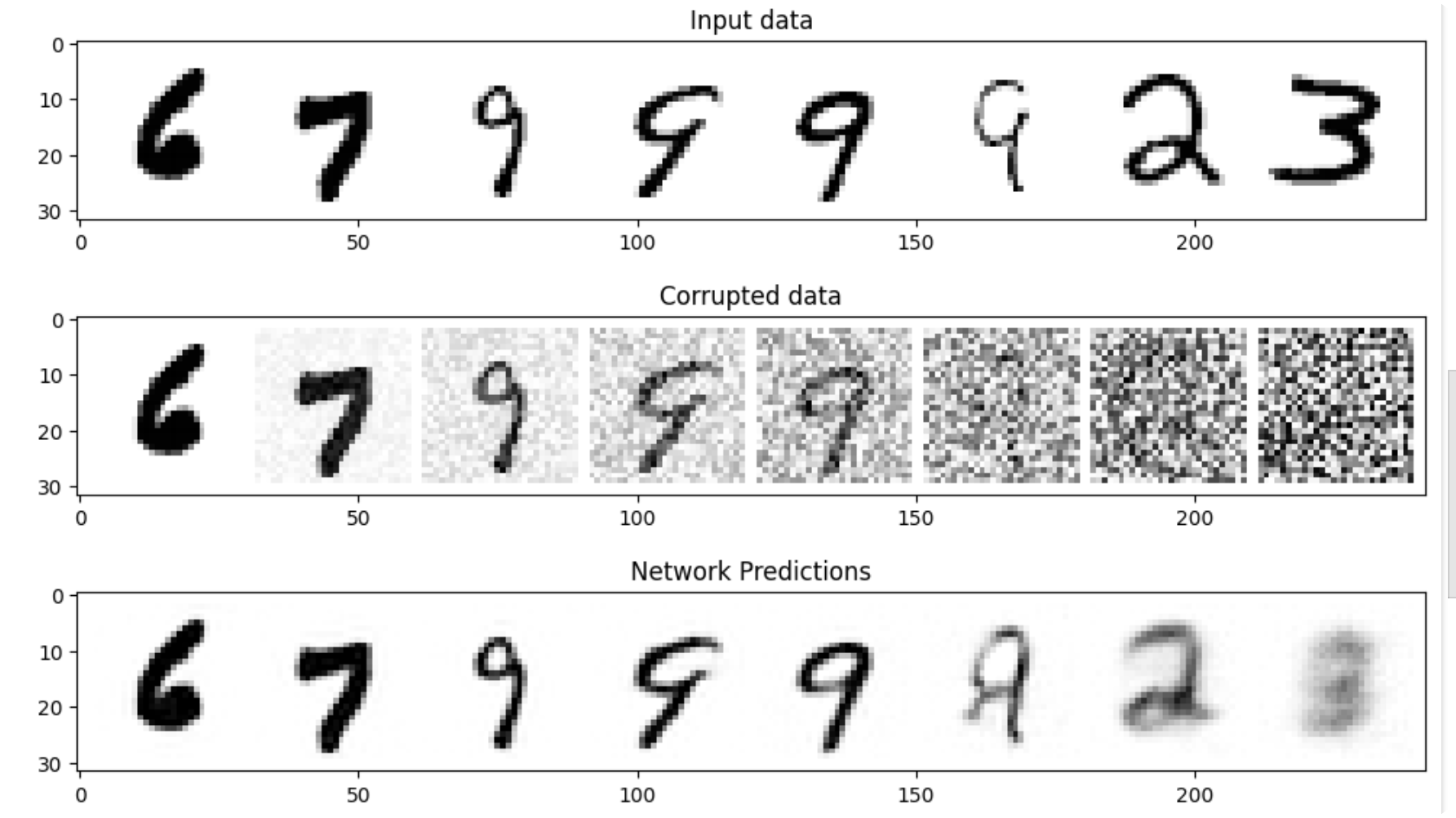
Though, for the image with higher noise-level(more like Gaussian Distribution), the network perform well. One small trick we can use it to pass the image through model several times. We hope each time, the predicted image will get better.

n_steps = 8
x = torch.rand(8, 1, 28, 28).to(device)
step_history = [x.detach().cpu()]
pred_output_history = []

for i in range(n_steps):
    with torch.no_grad():
        pred = net(x)

    step_history.append(x.detach().cpu())
    pred_output_history.append(pred.detach().cpu())
    mix_factor = 1 / (n_steps - i)
    x = x * (1 - mix_factor) + pred * mix_factor

After we pass the model 8 times, we get the result:

Figure 3: The result of the pass model 8 times. On the left of the row is the input to the model and on the right is the denoised images

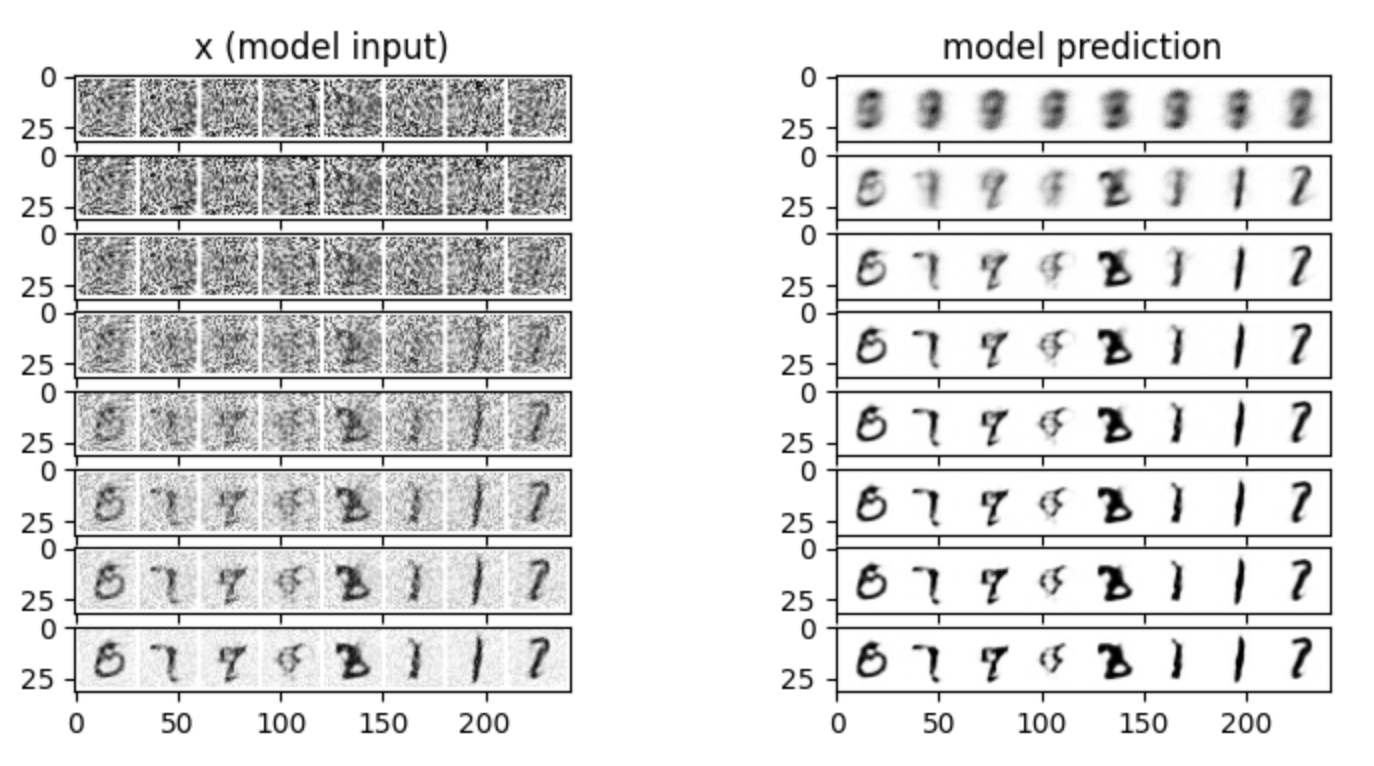
It shows that the output truly get better each times.

We increase the number of steps, the result will get better. Below is how it look like after we pass the model 40 times.

Figure 4: The result of passing model 40 times

Summary for now

In the above example, we see how the Diffusion Model work, we first corrupt the images, and then pass the pass the corrupted images to the model to get the de-noised images back. We training the the model using Mean Square Loss Equation 1. To improve the quality of sampling, we can pass the out back to the model several times Figure 3. The Full code is available here

Diffusion Model for Discrete Data

Recently, there are some good exploration for the diffusion model when apply on the. For example, Inception is the first commercial-scale diffusion language model. Which is is faster than the general language model.

References

Ronneberger, Olaf, Philipp Fischer, and Thomas Brox. 2015. “U-Net: Convolutional Networks for Biomedical Image Segmentation.” May 18, 2015. https://doi.org/10.48550/arXiv.1505.04597.